We say, one image worth 1000 words. Similarly visual representations are sometimes more meaningful than raw data. Conditional formatting is a life saving feature we find in spreadsheets. It allows to format cells based on some condition. In MS Excel, conditional formatting allows background colors, data bars, color scales and icon sets. Among all, icon sets is a cool feature which allows to display various icons in a cell according to condition.  
In Google Spreadsheet, conditional formatting allows background and font formatting, icon sets are not yet supported. But there is a workaround which can help you to apply different icons based on condition similar to MS Excel icon sets.

How it works ?

We can apply following two formula combinedly to achieve the similar feature.

1. IF(logical_expression, value_if_true, value_if_false) 
2. IMAGE(url, [mode], [height], [width]) 

You can upload your icons in any server or any 3rd party sites available on internet. Then apply your formula as shown in below example. 

=IF(A3<50,IMAGE("your_icon_url",3),IMAGE("your_icon_url",3)) 

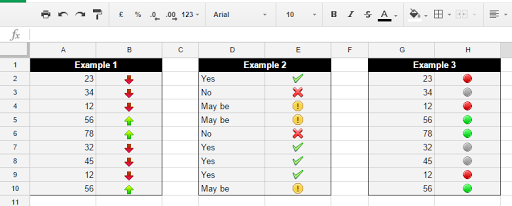
Above formula will render two different images based on the condition A3<50 
You can even use nested IF when you have more than 2 conditions. Here is an example: 

=IF(D2="Yes",IMAGE("your_icon_url",3),IF(D2="No",IMAGE("your_icon_url",3),IMAGE("your_icon_url",3))) 

Above formula will show three different icons based on the cell value "Yes", "No" and "May be". You can also mark the nested IF present in place of ELSE of first IF. Here is an example worksheet to play around.

Demo

Bonus tips 

• You can check in the formula IMAGE("your_icon_url",3) contains a 2nd parameter 3. It is an optional parameter and indicates the sizing mode of the icon. So, 3 is to display the original size of the icon. This way you can ensure that the icon rendering will not stretch size or look blur. 

• If you are playing with cells which contains letters then it is better to wrap the cell value with LOWER(text), so that it can handle both upper and lowercase letters. For example, "YES" and "yes". 

• In MS Excel there is an option to "show only icons", which will hide the textual data and display only the icon in the cell. Though there is no direct way to achieve this in Google Spreadsheet but you can always hide the textual column to get the same type of experience.